Approaching the Edge of Decision

TL;DR Complex data does not equate a complex classification problem. In order to change the outlook from data-driven to task-oriented we must first accurately, define sample and characterize the decision boundary of a given problem.

Prelude

_Complex data requires complex models._ Or so the saying goes. In every domain, one of the major difficulties is selecting the optimal model architecture for given a classification problem. Most approaches tend to be domain-specific [reference] or offer no reasonable explanations of a model's architecture choice, aside from superior performance [references]. The only logical step would be to look at the data itself [^1] and build a model based of certain characteristics of the data. But what is complex data anyways? If we follow [Will] then complex data is data that has _non-trivial homology_ . However, classifying two concentric circles is challenging not because they are circles, but because they are concentric.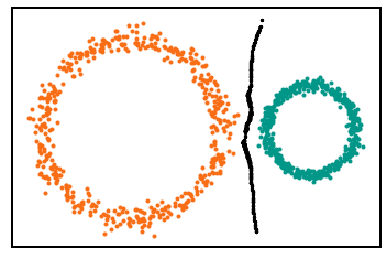

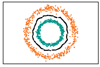
The data in both problems has exactly the same topological characteristics. Yet it would be reckless to assume both tasks are equivalent. One is linearly separable (left) while the other clearly isn’t. We intuitively understand that we would require a more complex model to differentiate the classes in the right. Or better yet, only a more complex problem could.

Is there a way to measure this? Can we formalize a new method somehow? Well the answer becomes quite simple, if one believes in the idea of entanglement ¹. It would go something along the lines of:

• Measure the entanglement of the classes, given by the homology of its decision boundary.
• Understand how a model’s architecture affects the homology of the decision boundary it expresses.

There are so many problems just in the first line, including, but not limited to: What is a decision boundary? Is it a decision boundary or the decision boundary? Isn’t finding its homology the same as solving a classification problem?…

In this post we will go over all these problems, but just the ones regarding the first point on the list. The second one is much more lengthy, ambiguous, and, honestly, more of a Fermat’s-last-theorem kind of problem.

Overture

Before we get rigorous we should start defining some things here[^7]. The idea is to build upon our intuition of characterizing how complex a _problem_ actually is. In the *Prelude* we talked about how one of the problems was linearly separable [image]. Because we can separate both classes with a straight line. A linearly separable problem in 3 dimensions could be separated with a plane, and so forth. This separating hyperplane we call decision boundary:

Definition 1.1 We call decision boundary of $\mathbb{R}^n$ to a $n-1$ dimensional manifold that separates the space in $c$-classes.

Definition 1.2 We say that manifolds are linearly separable if their decision boundary is a plane.

Obviously the decision boundary in not unique. It can be, but most cases it isn’t. So which one do we consider? Well the most intuitive and broad would be to consider the decision boundary that maximizes the distance between any 2 points of different classes. This one is unique though, and we can actually define it very well, but first.

Definition 1.3 (Voronoi cover) For each point in ${R}^n$ in a given set $S = {s_1, …, s_k}$ we define a Voronoi cell as the set: $$ x \in V_{s_i} \quad \Leftrightarrow \quad d(x,s_i)\leq d(x, s_j) \quad \forall x\in\mathbb{R}^n \land i\neq j $$ We call **Voronoi cover** to the cover $V_S = (\mathcal{V}_\sigma)_{\sigma \in S}$

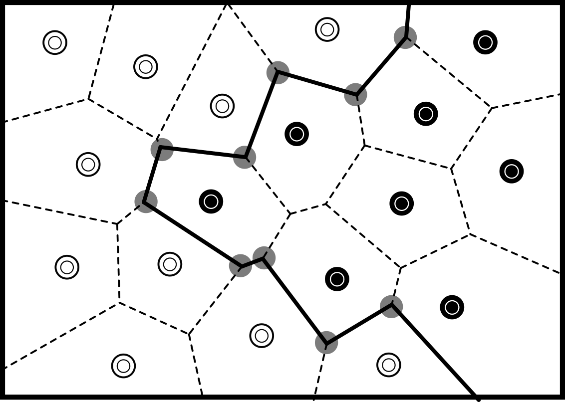
A Voronoi cover simple partitions the space into cells of points that are “the closest” to a predefined point (our data point). Now consider a Voronoi cover with points of different classes, if we take two adjacent cells of points of different classes say point $a$ and $b$, the common edge $E_{ab}$ of that cell is made of the points that:

• Are the same distance to $a$ and $b$, $$ x \in R^n \mid d(x,a)=d(x,b) $$

• Both $a,b$ are the closest of all data points (definition of Voronoi):

$$ E_{ab}={x\in R^n \mid d(x,a) = d(x,b) \leq d(x,s) \forall s\notin {a,b}} $$

If we take the union of these edges of all adjacent pairs of different classes we have the decision boundary.

Definition 1.4 We call Voronoi Decision Boundary (or just decision boundary) to the union $$ DB = \bigcup E_{a,b} \quad \forall (a,b) \in Adj $$ Where $Adj$ is the set of ordered pairs $(a_i,b_i)$ where $a_i$ and $b_i$ belong to different classes and their Voronoi cells are adjacent.

Ok, now just like no one really cares about a TDA implementation on github that doesn’t work above 3 dimensions, the Voronoi and Delaunay should also invoke to you some high-dimensional dread. Because, truth is, the calculation of Voronoi cover in high dimensions is prohibitive.

There is a workaround. We don’t need all of the Voronoi cover, just the ability to sample points from the union of some of its edges. Thus, not having to calculate intersections should throw us to sub-quadratic running time, hopefully.

Algorithm 1.5 Sample decision boundary.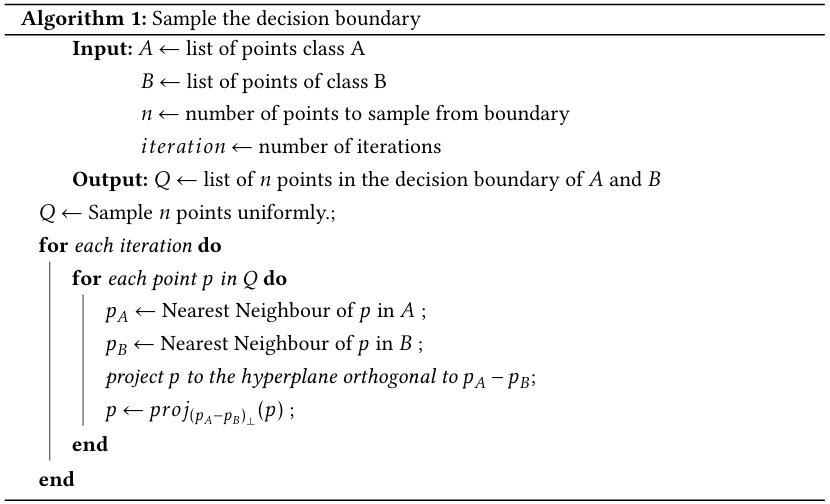

• Cover the space with a set $Q$ of uniformly sampled points.

Repeat for number_of_iterations:

• For each point $q$ in $Q$ find its closest points of different classes $a,b$
• Project $q$ to the affine hyperspace orthogonal to $a-b$

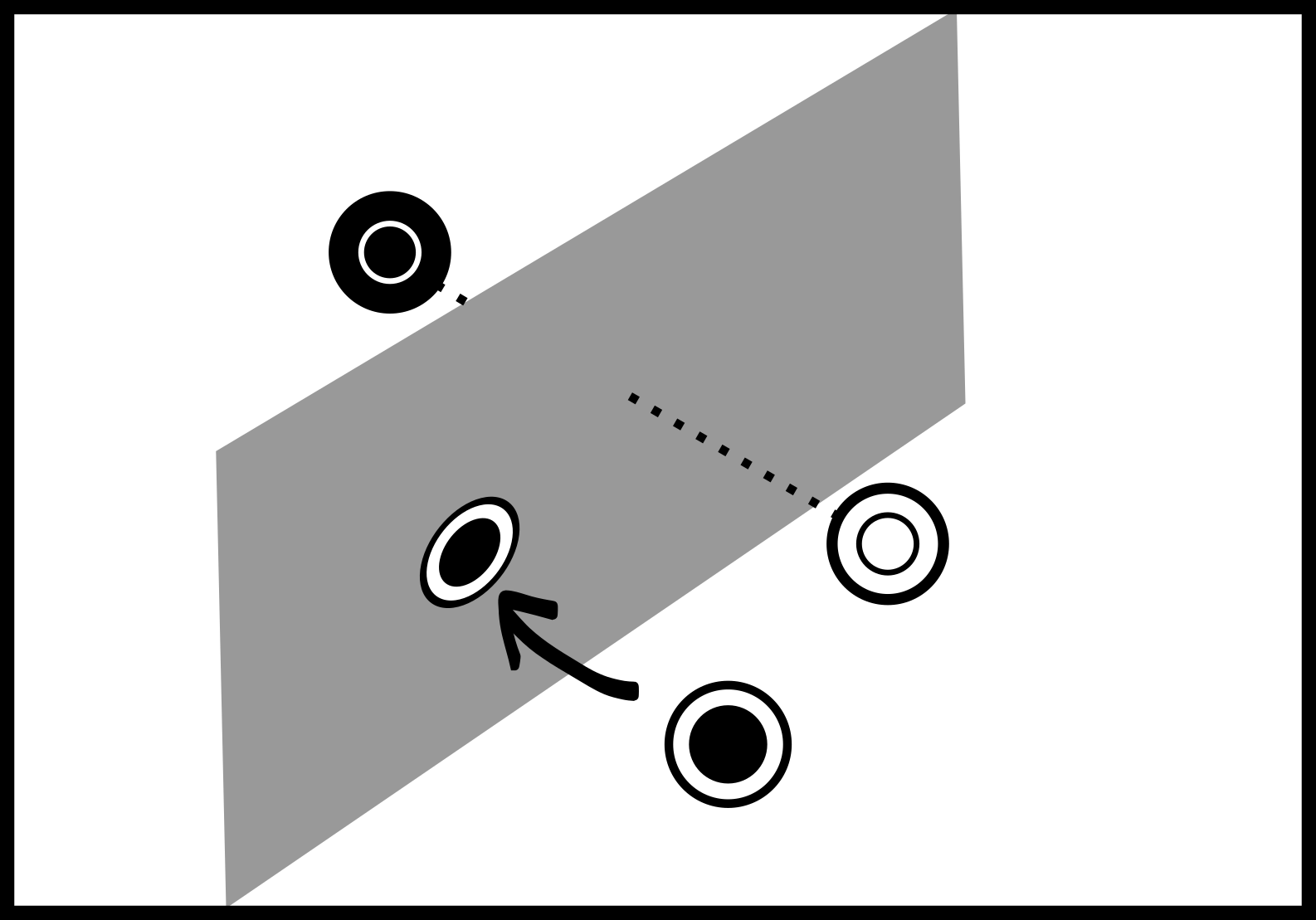
The fact is, the algorithm works by “pushing” each point in the cover $Q$ towards the boundary by projecting it to these “sub-boundaries”. If, at a given iteration $(a,b) \notin Adj$ then $a,b$ are no longer the closest points of different classes. Basically, the only stationary points of this process are the points in the voronoi decision boundary.

Proposition 1.6 The algorithm converges to the Voronoi edges of adjacent cells of points of different classes.

Proof. By definition the Voronoi cell associated with point $s_i \in S$ is the set ${x\in \mathbb{R}^n \mid d(x,s_i) \leq d(x,s_j) \forall i\neq j}$. Given a point $a_i$ belonging to a class, and $b_i$ belonging to another class, we have that the set of points in the common edge of their Voronoi cells is given by: $$ DB_{ab} = {x\in\mathbb{R}^n\mid d(x,a_i)=d(x,b_i)\leq d(x,s_j)} $$ Therefore, at a given iteration of the algorithm, if point $q$ does not belong to the set $DB_{ab}$ then, by definition of Voronoi cell, there has to exist a point $a_j$ (or $b_j$) such that $d(q,a_j) < d(q,a_i)=d(q,b_i)$. And therefore this point is considered the new closest neighbor in the next iteration. It follows that the algorithm only stops when all points reach the decision boundary. _(End of proof)_

---

1. Yes, I say believe since it is not really a defined thing in topology. Which also means we can define it as whatever we want. Basically I’m not asking you to believe in entanglement, I’m asking you to believe me. ↩︎